Application Case 2.2
Improving Student Retention with Data-Driven Analytics
Student attrition has become one of the most challenging problems for decision makers in academic institutions. Despite all the programs and services that are put in place to help retain students, according to the U.S. Department of Education, Center for Educational Statistics (nces.ed.gov), only about half of those who enter higher education actually earn a bachelor’s degree. Enrollment management and the retention of students has become a top priority for administrators of colleges and universities in the United States and other countries around the world. High dropout of students usually results in overall financial loss, lower graduation rates, and inferior school reputation in the eyes of all stakeholders. The legislators and policy makers who oversee higher education and allocate funds, the parents who pay for their children’s education to prepare them for a better future, and the students who make college choices look for evidence of institutional quality and reputation to guide their decision-making processes.
Proposed Solution
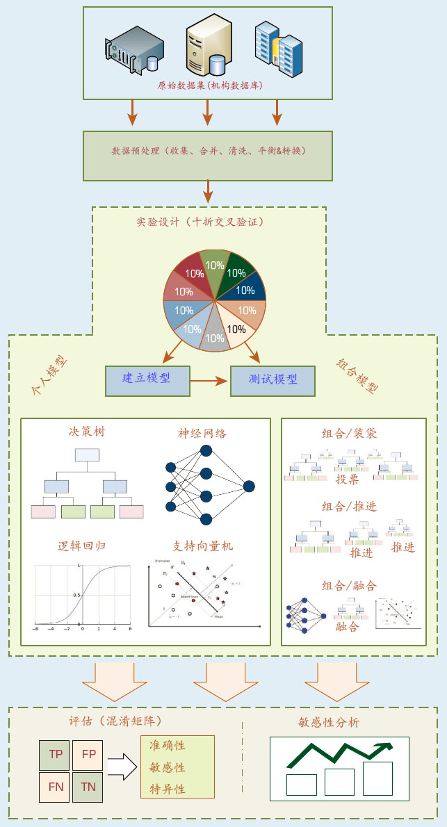
To improve student retention, one should try to understand the nontrivial reasons behind the attrition. To be successful, one should also be able to accurately identify those students that are at risk of dropping out. So far, the vast majority of student attrition research has been devoted to understanding this complex, yet crucial, social phenomenon. Even though these qualitative, behavioral, and survey-based studies revealed invaluable insight by developing and testing a wide range of theories, they do not provide the much-needed instruments to accurately predict (and potentially improve) student attrition. The project summarized in this case study proposed a quantitative research approach where the historical institutional data from student databases could be used to develop models that are capable of predicting as well as explaining the institution-specific nature of the attrition problem. The proposed analytics approach is shown in Figure 2.4.
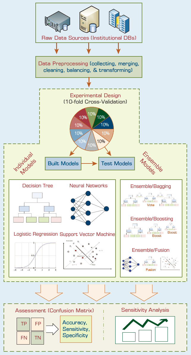
FIGURE 2.4 An Analytics Approach to Predicting Student Attrition.
Although the concept is relatively new to higher education, for more than a decade now, similar problems in the field of marketing management have been studied using predictive data analytics techniques under the name of “churn analysis,” where the purpose has been to identify among the current customers to answer the question, “Who among our current customers are more likely to stop buying our products or services?” so that some kind of mediation or intervention process can be executed to retain them. Retaining existing customers is crucial because as we all know, and as the related research has shown time and time again, acquiring a new customer costs on an order of magnitude more effort, time, and money than trying to keep the one that you already have.
Data Is of the Essence
The data for this research project came from a single institution (a comprehensive public university located in the Midwest region of the United States) with an average enrollment of 23,000 students, of which roughly 80% are the residents of the same state and roughly 19% of the students are listed under some minority classification. There is no significant difference between the two genders in the enrollment numbers. The average freshman student retention rate for the institution was about 80%, and the average 6-year graduation rate was about 60%.
The study used 5 years of institutional data, which entailed to 16,000+ students enrolled as freshmen, consolidated from various and diverse university student databases. The data contained variables related to students’ academic, financial, and demographic characteristics. After merging and converting the multidimensional student data into a single flat file (a file with columns representing the variables and rows representing the student records), the resultant file was assessed and preprocessed to identify and remedy anomalies and unusable values. As an example, the study removed all international student records from the data set because they did not contain information about some of the most reputed predictors (e.g., high school GPA, SAT scores). In the data transformation phase, some of the variables were aggregated (e.g., “Major” and “Concentration” variables aggregated to binary variables MajorDeclared and ConcentrationSpecified) for better interpretation for the predictive modeling. In addition, some of the variables were used to derive new variables (e.g., Earned/Registered ratio and YearsAfterHighSchool).
Earned/Registered = EarnedHours/ RegisteredHours
YearsAfterHighSchool = FreshmenEnrollmentYear – HighSchoolGraduationYear
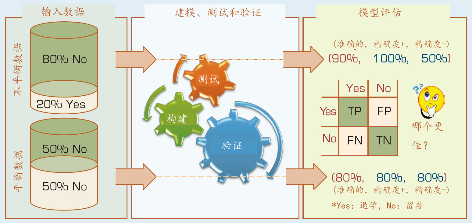
The Earned/Registered ratio was created to have a better representation of the students’ resiliency and determination in their first semester of the freshman year. Intuitively, one would expect greater values for this variable to have a positive impact on retention/ persistence. The YearsAfterHighSchool was created to measure the impact of the time taken between high school graduation and initial college enrollment. Intuitively, one would expect this variable to be a contributor to the prediction of attrition. These aggregations and derived variables are determined based on a number of experiments conducted for a number of logical hypotheses. The ones that made more common sense and the ones that led to better prediction accuracy were kept in the final variable set. Reflecting the true nature of the subpopulation (i.e., the freshmen students), the dependent variable (i.e., “Second Fall Registered”) contained many more yes records (~80%) than no records (~20%; see Figure 2.5).
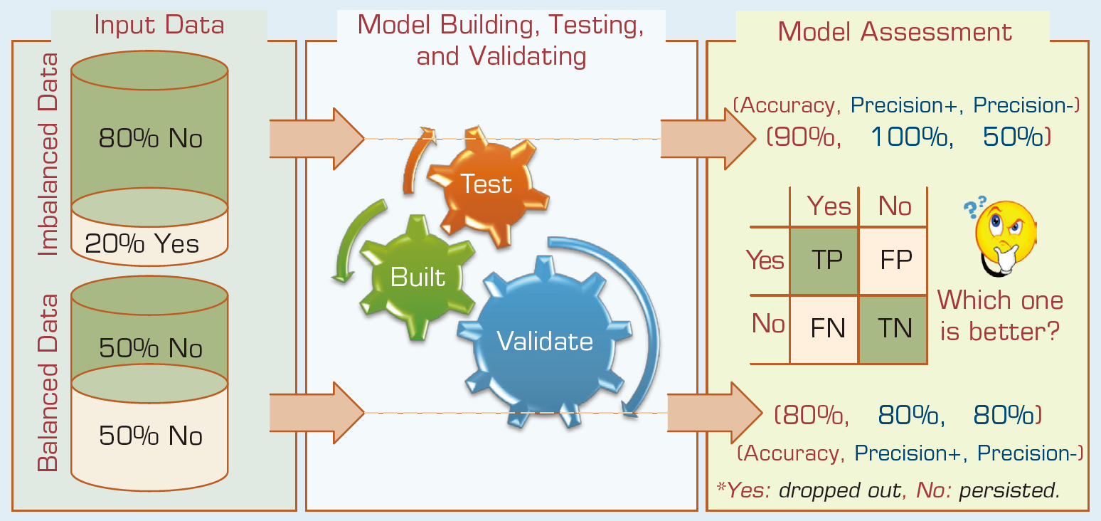
FIGURE 2.5 A Graphical Depiction of the Class Imbalance Problem.
Research shows that having such an imbalanced data has a negative impact on model performance. Therefore, the study experimented with the options of using and comparing the results of the same type of models built with the original imbalanced data (biased for the yes records) and the wellbalanced data.
Modeling and Assessment
The study employed four popular classification methods (i.e., artificial neural networks, decision trees, support vector machines, and logistic regression) along with three model ensemble techniques (i.e., bagging, busting, and information fusion). The results obtained from all model types were then compared to each other using regular classification model assessment methods (e.g., overall predictive accuracy, sensitivity, specificity) on the holdout samples.
In machine-learning algorithms (some of which will be covered in Chapter 4), sensitivity analysis is a method for identifying the “cause-and-effect” relationship between the inputs and outputs of a given prediction model. The fundamental idea behind sensitivity analysis is that it measures the importance of predictor variables based on the change in modeling performance that occurs if a predictor variable is not included in the model. This modeling and experimentation practice is also called a leave-one-out assessment. Hence, the measure of sensitivity of a specific predictor variable is the ratio of the error of the trained model without the predictor variable to the error of the model that includes this predictor variable. The more sensitive the network is to a particular variable, the greater the performance decrease would be in the absence of that variable, and therefore the greater the ratio of importance. In addition to the predictive power of the models, the study also conducted sensitivity analyses to determine the relative importance of the input variables.
Results
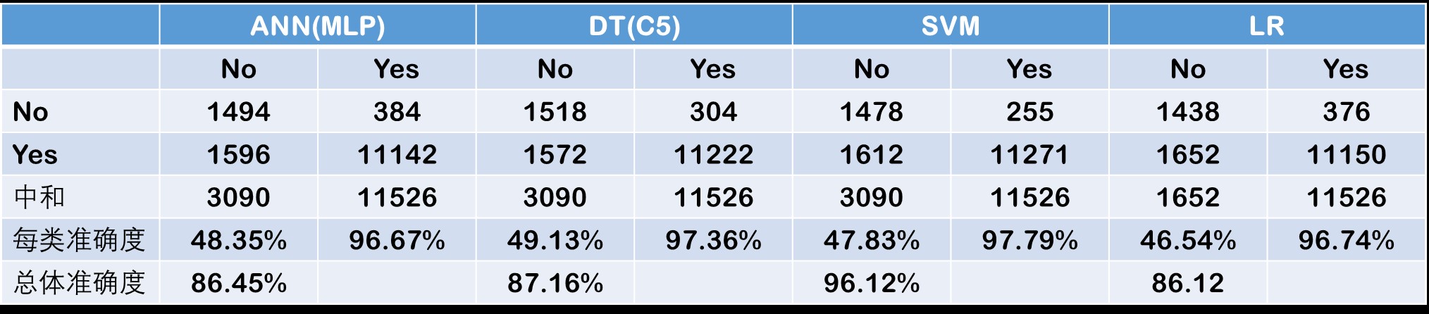
In the first set of experiments, the study used the original imbalanced data set. Based on the 10-fold cross-validation assessment results, the support vector machines produced the best accuracy with an overall prediction rate of 87.23%, the decision tree came out as the runner-up with an overall prediction rate of 87.16%, followed by artificial neural networks and logistic regression with overall prediction rates of 86.45% and 86.12%, respectively (see Table 2.2). A careful examination of these results reveals that the predictions accuracy for the “Yes” class is significantly higher than the prediction accuracy of the “No” class. In fact, all four model types predicted the students who are likely to return for the second year with better than 90% accuracy, but they did poorly on predicting the students who are likely to drop out after the freshman year with less than 50% accuracy. Because the prediction of the “No” class is the main purpose of this study, less than 50% accuracy for this class was deemed not acceptable. Such a difference in prediction accuracy of the two classes can (and should) be attributed to the imbalanced nature of the training data set (i.e., ~80% “Yes” and ~20% “No” samples).
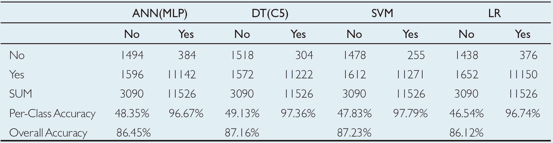
TABLE 2.2 Prediction Results for the Original/Unbalanced Dataset
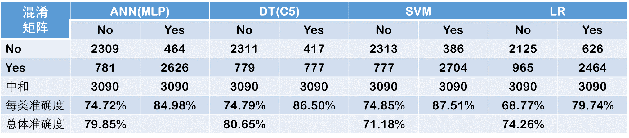
The next round of experiments used a wellbalanced data set where the two classes are represented nearly equally in counts. In realizing this approach, the study took all the samples from the minority class (i.e., the “No” class herein) and randomly selected an equal number of samples from the majority class (i.e., the “Yes” class herein) and repeated this process for 10 times to reduce potential bias of random sampling. Each of these sampling processes resulted in a data set of 7,000+ records, of which both class labels (“Yes” and “No”) were equally represented. Again, using a 10-fold crossvalidation methodology, the study developed and tested prediction models for all four model types. The results of these experiments are shown in Table 2.3. Based on the holdout sample results, support vector machines once again generated the best overall prediction accuracy with 81.18%, followed by decision trees, artificial neural networks, and logistic regression with an overall prediction accuracy of 80.65%, 79.85%, and 74.26%. As can be seen in theper-class accuracy figures, the prediction models did significantly better on predicting the “No” class with the well-balanced data than they did with the unbalanced data. Overall, the three machine-learning techniques performed significantly better than their statistical counterpart, logistic regression.
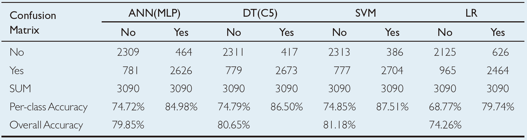
TABLE 2.3 Prediction Results for the Balanced Data Set
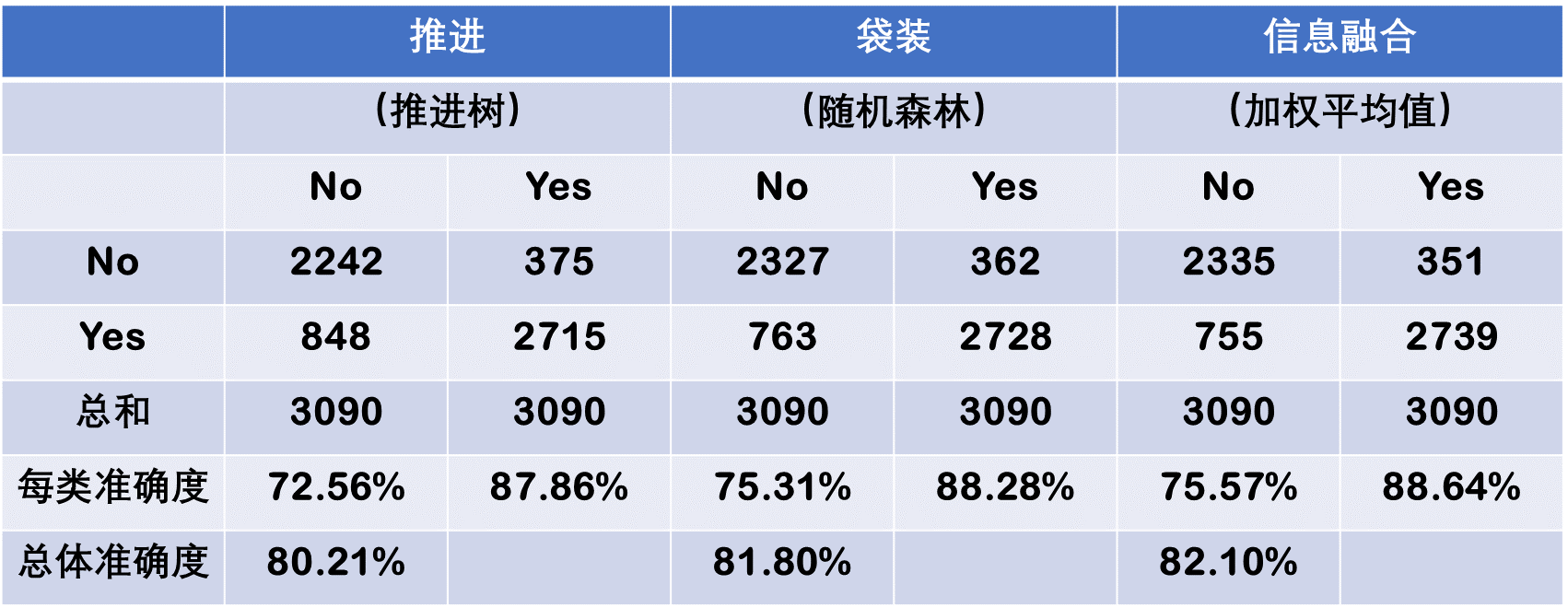
Next, another set of experiments were conducted to assess the predictive ability of the three ensemble models. Based on the 10-fold crossvalidation methodology, the information fusion–type ensemble model produced the best results with an overall prediction rate of 82.10%, followed by the bagging-type ensembles and boosting-type ensembles with overall prediction rates of 81.80% and 80.21%, respectively (see Table 2.4). Even though the prediction results are slightly better than the individual models, ensembles are known to produce more robust prediction systems compared to a single-best prediction model (more on this can be found in Chapter 4).
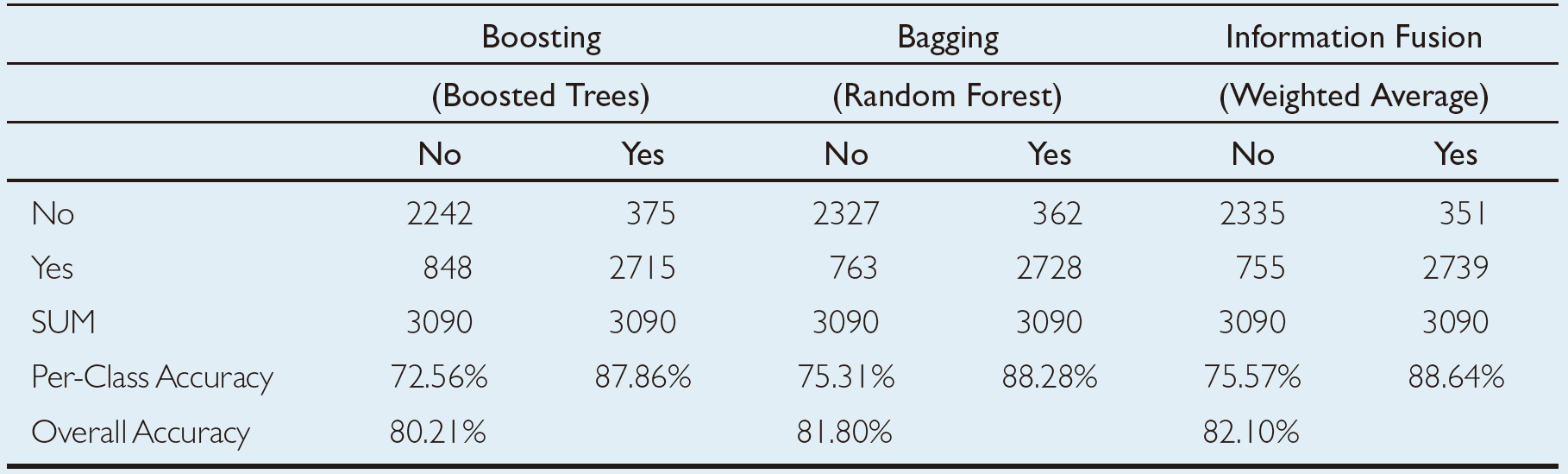
TABLE 2.4 Prediction Results for the Three Ensemble Models
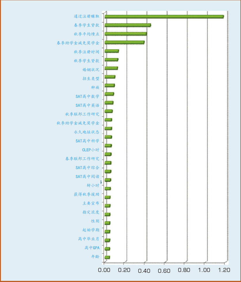
In addition to assessing the prediction accuracy for each model type, a sensitivity analysis was also conducted using the developed prediction models to identify the relative importance of the independent variables (i.e., the predictors). In realizing the overall sensitivity analysis results, each of the four individual model types generated its own sensitivity measures ranking all the independent variables in a prioritized list. As expected, each model type generated slightly different sensitivity rankings of the independent variables. After collecting all four sets of sensitivity numbers, the sensitivity numbers are normalized and aggregated and plotted in a horizontal bar chart (see Figure 2.6).
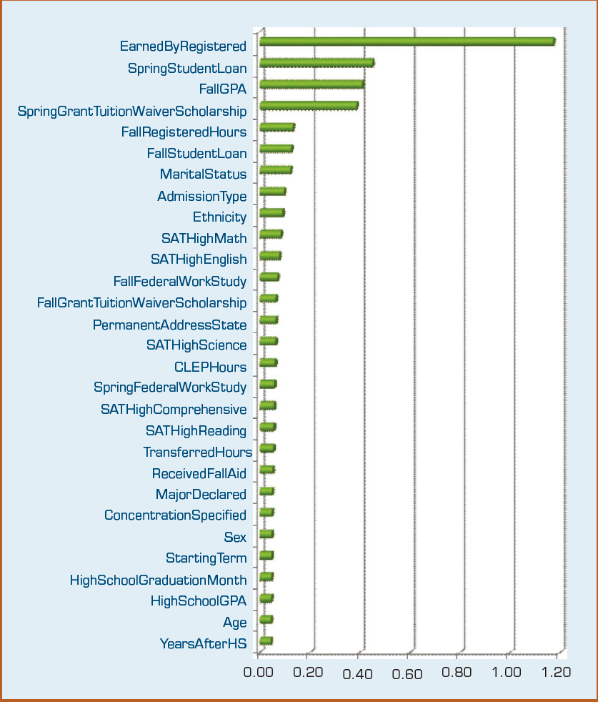
FIGURE 2.6 Sensitivity-Analysis-Based Variable Importance Results.
Conclusions
The study showed that, given sufficient data with the proper variables, data mining methods are capable of predicting freshmen student attrition with approximately 80% accuracy. Results also showed that, regardless of the prediction model employed, the balanced data set (compared to unbalanced/ original data set) produced better prediction models for identifying the students who are likely to drop out of the college prior to their sophomore year. Among the four individual prediction models used in this study, support vector machines performed the best, followed by decision trees, neural networks, and logistic regression. From the usability standpoint, despite the fact that support vector machines showed better prediction results, one might choose to use decision trees because compared to support vector machines and neural networks, they portray a more transparent model structure. Decision trees explicitly show the reasoning process of different predictions, providing a justification for a specific outcome, whereas support vector machines and artificial neural networks are mathematical models that do not provide such a transparent view of “how they do what they do.”